Support Vector Regression
June 8, 2021
Support vector machines (SVM) are usually explained through a binary classification point of view. But recently, I find out you can also use SVM for regression [1]. And I find it so much easier to understand.
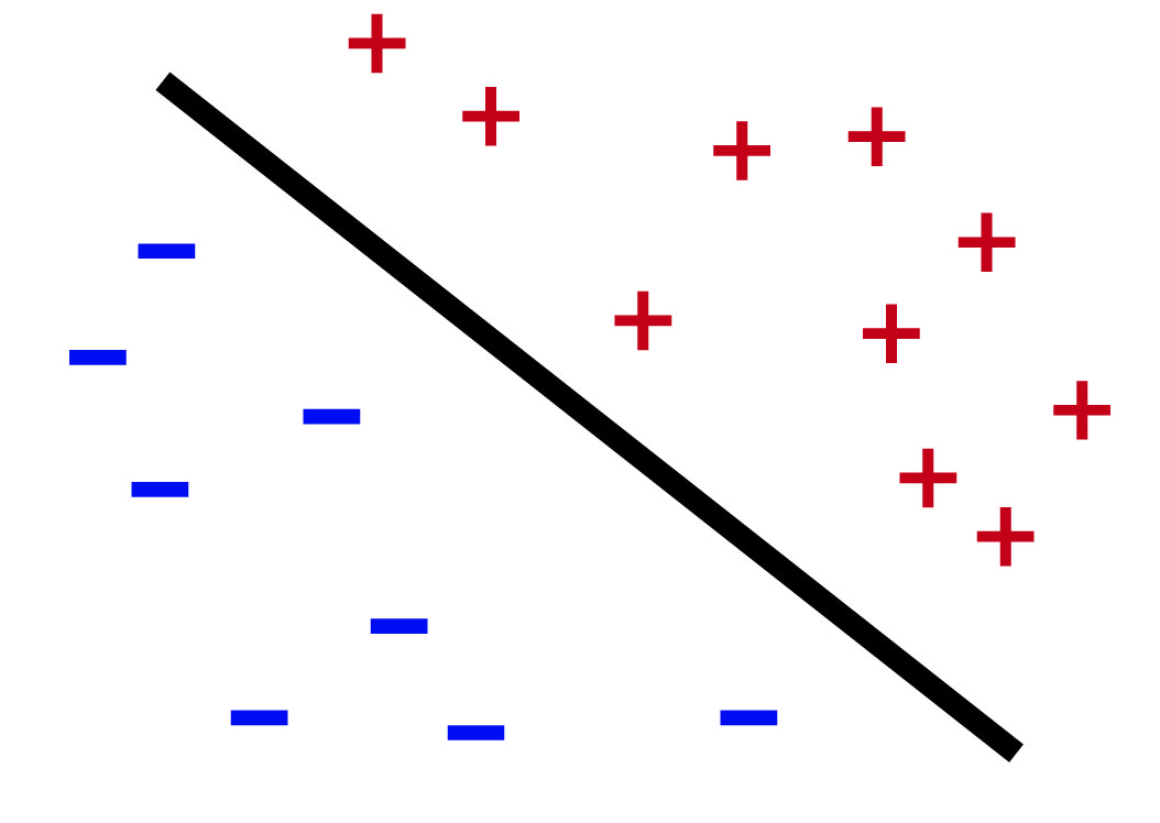
Instead of a picture with a hyperplane separating pluses and minuses for binary classification like this:
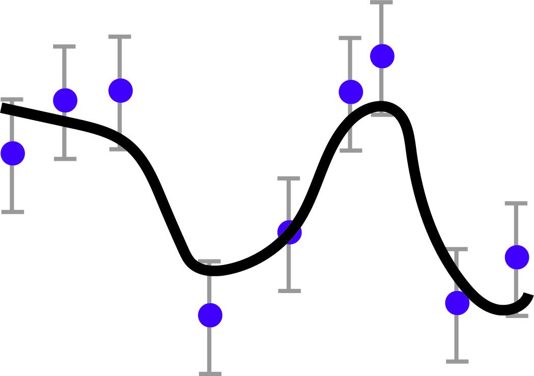
The regression picture becomes a curve fitting through data points like this:
In the following, I will go through SVM for regression, also known as SVR. I will do so in the kernel regression framework, which makes the formulation extremely simple. The derivation will also show a connection to \(\ell 1\) regularized regression, which links support vectors to sparsity. Finally, I will formulate SVM for binary classification in the same framework.
Problem Setup
We have training data points \((x_1, y_1), \ldots, (x_n, y_n).\) They can be scalars, vectors, real-valued or complex valued. Our goal is to fit a function \(f(x)\) to the data points.
Because the data points may have some noise, we only want the function to approximate them. SVR considers a very particular loss function: a uniform error bound with a tolerance \(\epsilon\), that is \[ | f(x_i) - y_i | \leq \epsilon, \] for \(i = 1, \ldots, n\).
Kernel Regression
There are infinitely many ways to fit a curve to finitely many points, so we need to somehow restrict the problem. The kernel regression way is to constrain the function to be in a "kernel space".
At a high level, a kernel function takes two inputs, and outputs a scalar. You can think of a kernel function as a similarity function that measures how similar the two inputs are. A "kernel space" contains all linear combination of kernel functions with one input fixed at different locations. Pictorially, a function from the "kernel space" looks something like this:
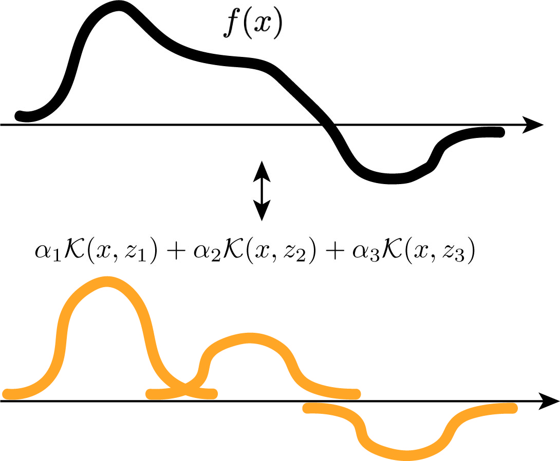
Concretely, given a positive semi-definite kernel \(\mathcal{K}(x, x')\), we can construct a corresponding reproducible kernel Hilbert space (RKHS) \(\mathbb{H}\) by taking every linear combination of kernel functions like this, \[ f(x) = \sum_{i = 1}^n \alpha_i \mathcal{K}(x, x_i), \] and their limits. With appropriate technicalities, this construction surprisingly induces an inner product \(\langle f, g \rangle\) and a norm \(\| f \|_\mathbb{H} = \sqrt{\langle f, f \rangle} \) in the function space. Which makes it a Hilbert space.
SVR
In SVR, we have the error constraints \(|f(x_i) - y_i| \leq \epsilon\). And to regularize the problem, we minimize the norm of the function \(\| f \|_{\mathbb{H}}\). Putting things together, we have the following regression problem: \begin{align} &\min_{f \in \mathbb{H}} &&\| f \|_{\mathbb{H}}\\ &\text{s.t.} && |f(x_i) - y_i| \leq \epsilon \end{align} for \(i = 1, \ldots, n.\)
And that's it. This is the optimization problem for SVR. It is not the most general form. Some people call it "\(\epsilon\)-insensitive support vector regression" [1]. But it is still an SVR. Conceptually, it is simple. We want to fit a function to data points with minimum norm under some error tolerance.
Dual Problem
We are not done yet because the optimization variable is a function and we cannot solve it on a computer. To turn it into a finite optimization problem, we can look at its dual form.
To derive the dual problem, we will use the following RKHS property: Evaluating an RKHS function \(f\) at any point \(x'\) is an inner product operation, that is, \[ f(x') = \langle f, \mathcal{K}(x, x') \rangle. \]
This basically transforms our function fitting problem to a linear inverse problem in the function space. \(f(x_i) = y_i\) now becomes a linear equation \(\langle f, \mathcal{K}(x, x_i) \rangle = y_i\).
Next, we derive the dual problem with the Lagrangian formulation. We split the error constraints into upper and lower bound and assign \(\alpha^+_i\) and \(\alpha^-_i\) as their Lagrangian variables. Then we have the following Lagrangian formulation: \begin{align} &\min_{f} \max_{\alpha^{+}_i \geq 0, \alpha^{-}_i \geq 0} \frac{1}{2}\| f \|_{\mathbb{H}}^2 \\ &- \sum_{i = 1}^n \alpha_i^+ (\langle f, \mathcal{K}(x, x_i) \rangle - y_i - \epsilon) \\ &- \sum_{i = 1}^n \alpha_i^- (-\langle f, \mathcal{K}(x, x_i) \rangle + y_i - \epsilon) \end{align}
The dual problem simply switches the \(\min\) with the \(\max\). To solve for the inner minimization problem, we set the derivative with respect to \(f\) to zero. Rearranging, we obtain \[ f - \sum_{i = 1}^n \alpha_i^+ \mathcal{K}(x, x_i) + \sum_{i = 1}^n \alpha_i^- \mathcal{K}(x, x_i) = 0. \]
Because both \(\alpha^+_i\) and \(\alpha^-_i\) are both non-negative, we can define a new variable \(\alpha_i = \alpha^+_i - \alpha^-_i\). Substituting, we obtain \[ f = \sum_{i = 1}^n \alpha_i \mathcal{K}(x, x_i). \]
Plugging this back to the maximin problem, and observing that \(\alpha_i^+ + \alpha_i^- = | \alpha_i |\), we obtain the following dual problem \[ -\left(\min_{\boldsymbol{\alpha}} \frac{1}{2} \boldsymbol{\alpha}^\top \mathbf{K} \boldsymbol{\alpha} - \boldsymbol{\alpha}^\top \mathbf{y} + \epsilon \| \boldsymbol{\alpha}\|_1\right) \] where \(\boldsymbol{\alpha}\) is the vectorized dual variable. \(\mathbf{K}\) is the kernel matrix with \((\mathbf{K})_{ij} = \mathcal{K}(x_i, x_j)\), and \(\mathbf{y}\) is the vectorized output.
To summarize, we can solve for the dual variable with an \(\ell 1\) regularized regression problem. Then the resulting function simply uses the dual variable as coefficients with corresponding kernel functions.
Taking a step back, the \(\ell 1\) regularization makes sense because the loss function we used in the original problem is an \(\ell_\infty\) ball constraint. So its dual is an \(\ell 1\) penalty. The regularization also shows why SVM results are sparse. In fact, support vectors are just training data points \(x_i\) with non-zero coefficents \(\alpha_i\).
Connecting back to binary classification
How can we change our formulation for binary classification?
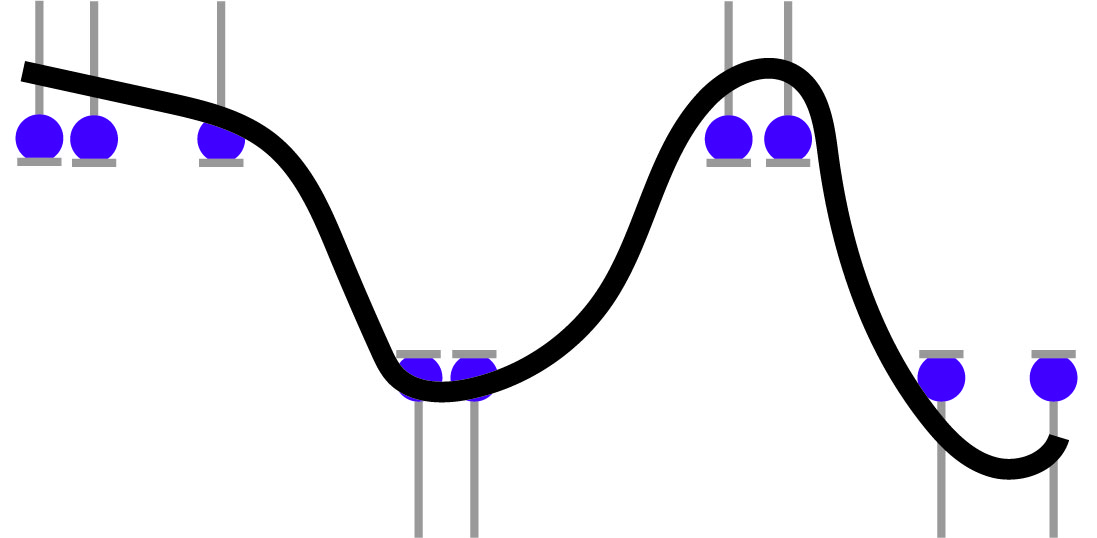
First, the data points only have two values, say \(\{+1, -1\}\). But that does not affect our optimization problem. The only change to the formulation is that we do not care how far the function extends beyond the label. The function only needs to get the signs correctly. So the picture becomes something like this:
Concretely, we have the following optimization problem \begin{align} &\min_{f \in \mathbb{H}} &&\| f \|_{\mathbb{H}}\\ &\text{s.t.} && f(x_i) \geq 1 - \epsilon, &&\text{if }y_i = 1,\\ & && f(x_i) \leq -1 + \epsilon, &&\text{if }y_i = -1, \end{align} for \(i = 1, \ldots, n.\)
Summary
I have shown a formulation of SVM for regression that is basically "fitting a curve through points with some error". To me, this is much simpler and easier to understand than the usual formulation of SVM for binary classification. The \(\ell 1\) regularization is also a nice connection.