The Burer-Monteiro factorization method [1, 2] is a powerful technique that can convert huge convex matrix problems into much smaller non-convex problems with optimality guarantees. At a high level, the method suggests that if you expect your solution to be of low rank, then you can solve for the low rank factors directly and check whether they are globally optimal.

In this post, I will go through one of the theoretical guarantees for smooth unconstrained minimization problems, following [3, 4]. As you will see, the proof is actually quite simple to follow.

Problem Setup

Concretely, we want to minimize a twice differentiable convex function \(f(\mathbf{X})\) over a positive semi-definite matrix \(\mathbf{X} \in \mathbb{C}^{n \times n}\): \[\min_{\mathbf{X} \succeq 0} f(\mathbf{X}).\]

We assume all optimal solutions have rank \(r\), much smaller than \(n\). This means \(\mathbf{X}\) can be factored as \(\mathbf{X} = \mathbf{U} \mathbf{U}^*\), where \(\mathbf{U}\) is an \(n \times r\) matrix, like this:

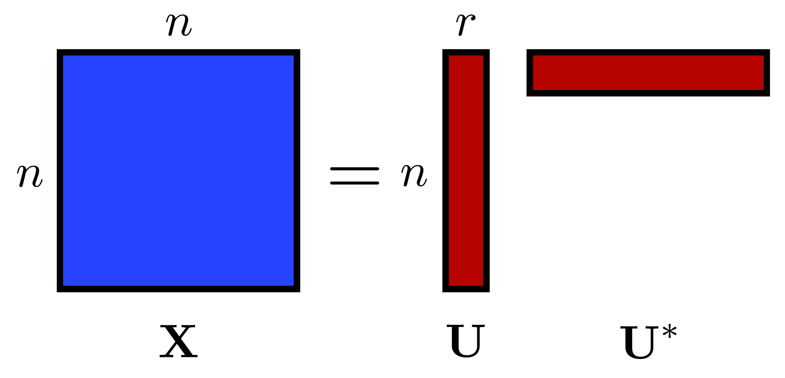
When \(n\) is large, it can be impractical to store and solve for the matrix \(\mathbf{X}\). Instead, the Burer-Monteiro factorization suggests solving directly for the low rank factors \(\mathbf{U}\). This results in \[ \min_{\mathbf{U}} g(\mathbf{U}) := f(\mathbf{U} \mathbf{U}^*). \] This problem is no longer convex, so it is not clear whether we can find a global optimum.

But we can still find something using iterative algorithms. In particular, it is still possible to solve for second-order stationary points (SOSPs), such that \begin{align} \nabla g(\mathbf{U}) &= 0 \\ \nabla^2 g(\mathbf{U}) &\succeq 0. \end{align}

Second-order methods naturally converge to SOSPs. And so do gradient descent with random initialization [5], and variants of stochastic gradient descent [6, 7].

But SOSPs are not necessarily global or even local optima. So to obtain optimality guarantees for these algorithms, our question becomes:

When does an SOSP coincide with a global minimum?

Main Result

The Burer Monteiro result says that an SOSP \(\mathbf{U}\) is optimal if \(\text{rank}(\mathbf{U}) \lt r\).

Notice the strict inequality. It is crucial to prescribe a rank that is bigger than the actual rank. In the proof, the rank deficiency will be used to select a vector in the null-space to cancel terms.

Proof

The proof consists of writing out the first-order optimality conditions of the convex problem. And matching to the second order stationary conditions of the non convex problem.

1. First Order Optimality Conditions

If there exists a matrix \(\mathbf{P}\) such that \begin{align} \mathbf{P} &\succeq 0, \\ \nabla f(\mathbf{X}) - \mathbf{P} &= 0, \\ \langle \mathbf{P}, \mathbf{X}\rangle &= 0, \\ \mathbf{X} &\succeq 0, \end{align} then \(\mathbf{X}\) is an optimal point of the convex problem.

The above conditions are known as the KKT conditions. And they can be simplified to: \begin{align}\langle\nabla f(\mathbf{X}), \mathbf{X}\rangle &= 0 \\ \nabla f(\mathbf{X}) &\succeq 0 \\ \mathbf{X} &\succeq 0 \end{align}

2. Linking the conditions

For any rank-deficient SOSP \(\mathbf{U}\), we want to show \(\mathbf{X} = \mathbf{U} \mathbf{U}^*\) is an optimal point to the original convex problem.

We first note that the condition \(\mathbf{X} \succeq 0\) is satisfied.

Let us then expand the second order optimality conditions. Using the chain rule, we obtain the following expression for the gradient: \[\nabla g(\mathbf{U}) = \nabla f(\mathbf{U} \mathbf{U}^*) \mathbf{U} = 0.\]

Taking the inner product on both sides with \(\mathbf{U}^*\) gives us \(\langle\nabla f(\mathbf{X}), \mathbf{X}\rangle = 0\).

Finally, let us look at the Hessian. \(\nabla^2 g(\mathbf{U}) \succeq 0\) means that for all \(\mathbf{V}\), we have, \[\nabla^2 g(\mathbf{U})[\mathbf{V}, \mathbf{V}] \geq 0.\]

If we expand it carefully using again the chain rule (Wikipedia provides a formula that is useful), we obtain, \[\text{tr}(\mathbf{V}^* \nabla f( \mathbf{U} \mathbf{U}^*) \mathbf{V}) + \nabla^2 f(\mathbf{U})[\mathbf{U} \mathbf{V}^* + \mathbf{V} \mathbf{U}^*][\mathbf{U} \mathbf{V}^* + \mathbf{V} \mathbf{U}^*] \geq 0.\]

Note that the first term is similar to what we want. Here’s where we use the fact \(\mathbf{U}\) is rank-deficient. In particular, we can choose \(\mathbf{V} = \mathbf{x} \mathbf{z}^*\) for any \(\mathbf{x}\), and for \(\mathbf{z}\) such that \(\|\mathbf{z}\|_2 = 1\) and \(\mathbf{z}\) is in the null space of \(\mathbf{U}\).

Since \(\mathbf{U} \mathbf{z}= 0\), the second term gets cancelled. Substituting \(\mathbf{V}\), and using \(\|\mathbf{z}\|_2 = 1\), we now have, \[\mathbf{x}^* \nabla f( \mathbf{U} \mathbf{U}^*) \mathbf{x} \geq 0,\] for all \(\mathbf{x}\). All three first-order optimality conditions are now satisfied, so \(\mathbf{X}=\mathbf{U} \mathbf{U}^*\) is optimal.

Extensions

To ensure the Burer-Monteiro factorization always works for a problem, the rank deficient condition must be shown to hold for all SOSPs. [4, 8, 9] showed that SOSPs for almost all linear objectives (ie \(g(\mathbf{U}) = \langle\mathbf{C}, \mathbf{U} \mathbf{U}^*\rangle\)) are low rank, so we can always choose a large enough \(r\).

For constrained problems, the proof is quite similar, but constraint qualifications on the non-convex problem are additionally needed. While they are commonly assumed in non-convex optimization algorithms, I often find them difficult to check in practice.

Nonetheless, the thing I like about Burer-Monteiro factorization technique is that it can provide a certificate in practice to check whether I have reached an optimal point. And this is still true for constrained problems.

References

1. S. Burer and R. D. C. Monteiro, “A nonlinear programming algorithm for solving semidefinite programs via low-rank factorization,” Mathematical Programming, vol. 95, no. 2, pp. 329–357, Feb. 2003.
2. S. Burer and R. D. C. Monteiro, “Local Minima and Convergence in Low-Rank Semidefinite Programming,” Mathematical Programming, vol. 103, no. 3, pp. 427–444, Jul. 2005.
3. M. Journée, F. Bach, P.-A. Absil, and R. Sepulchre, “Low-Rank Optimization on the Cone of Positive Semidefinite Matrices,” SIAM Journal on Optimization, vol. 20, no. 5, pp. 2327–2351, Jan. 2010.
4. S. Bhojanapalli, N. Boumal, P. Jain, and P. Netrapalli, “Smoothed analysis for low-rank solutions to semidefinite programs in quadratic penalty form,” in Conference On Learning Theory, 2018, pp. 3243–3270.
5. J. D. Lee, I. Panageas, G. Piliouras, M. Simchowitz, M. I. Jordan, and B. Recht, “First-order methods almost always avoid strict saddle points,” Math. Program., Feb. 2019.
6. R. Pemantle, “Nonconvergence to Unstable Points in Urn Models and Stochastic Approximations,” Ann. Probab., vol. 18, no. 2, pp. 698–712, Apr. 1990.
7. R. Ge, F. Huang, C. Jin, and Y. Yuan, “Escaping From Saddle Points — Online Stochastic Gradient for Tensor Decomposition,” arXiv:1503.02101 [cs, math, stat], Mar. 2015.
8. N. Boumal, V. Voroninski, and A. S. Bandeira, “The non-convex Burer-Monteiro approach works on smooth semidefinite programs,” arXiv:1606.04970 [cs, math], Jun. 2016.
9. D. Cifuentes, “Burer-Monteiro guarantees for general semidefinite programs,” arXiv:1904.07147 [math], Apr. 2019.